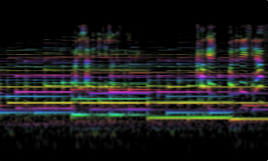
Chromatone Spectrogram

🌱 The Basics: See the Architecture of Sound

Chromatone Spectrogram is a real-time, colorized visual map of audio that runs directly in your browser. It translates the invisible physics of sound into a beautiful, readable landscape of color and light, allowing you to literally see the music.

How to use it:

1. Open the app and allow microphone access.
2. Play an instrument, sing, or play a song.
3. Watch the center line: new sounds appear instantly.
4. Notice the colors: each musical note has its own distinct color (A is red, B is bright yellow, F is deep blue).
5. Look at the edges: older sounds compress into deep "sediment" layers, revealing the overall structure and chord progressions of the song.
6. Use the camera and video buttons to capture your visualizations.

---

🧭 Core Philosophy & Approach

Moving beyond simple waveforms and standard mathematical spectrograms, this project treats music as a physical, geological phenomenon.

The Chromatone System We map the 12 notes of the chromatic scale to the 360 degrees of the color wheel. We intentionally use the HSL color space rather than perceptually uniform spaces (like OKLab) because the inherent "weight" and brightness of HSL colors carry emotional and pedagogical gravity. Yellow naturally radiates; blue recedes. This non-uniformity makes learning the "colors" of notes deeply intuitive and connects sound directly to human emotion.

The Cochleagram Standard spectrograms use linear or logarithmic math. We use a hybrid model that bridges musical theory (12-TET constant-Q) and human biology (cochlear Equivalent Rectangular Bandwidth). It visualizes sound not just as it exists in the air, but as it is perceived by the human ear.

Sedimentary Time Music is architecture experienced over time. By applying exponential time compression, we allow recent sounds to remain crisp and detailed, while older sounds compress into the background. This turns a fleeting audio stream into a readable "geological" record, where you can see the macro-structure, harmonic spread, and whistle tones of an entire song at a single glance.

---

✨ Key Features

• Deep Sediment Vision & Time Compression: Exponential scrolling that compresses deep history. Fast transients (snares, hi-hats) gracefully fade into the background over time, while sustained harmonic architecture remains vividly visible.
• Chromatone Frequency Mapping: Continuous 12-TET mapping where every A is red, cycling through the spectrum. Lower octaves are darker, higher octaves are lighter.
• Sub-Pixel Parabolic Peak Recovery: Recovers energy that falls between discrete FFT bins, making low notes tighter and high harmonics razor-sharp.
• Spectral Envelope Contrast: Removes cloudy "formant haze" and room resonances, leaving only the crisp, distinct harmonic partials.
• Transient / Sustained Separation: A dual-channel GPU architecture that independently tracks fast percussive attacks and slow harmonic sustains for perfect deep-time rendering.
• 2D Ridge-Aware Sharpening: Anisotropic Laplacian filtering in the shader that sharpens both horizontal harmonic ridges and diagonal pitch-bends without temporal ringing.
• Cochlear/Musical Hybrid Bands: Blends Constant-Q musical bands with ERB auditory filters from A0 to C9.
• Perceptual dB Pipeline: True logarithmic processing with A-weighting and pre-emphasis.
• Lateral Inhibition: On-center/off-surround spectral sharpening mimicking basilar membrane hair cells.
• Display P3 & High-Res Capture: Wide-gamut color support and high-quality video/screenshot recording.
• Zero-dependency PWA: Pure Web Audio API and WebGL2, installable and works offline.

---

⚙️ Technical Design & Mathematical Foundations

The rendering pipeline is divided into a highly optimized CPU-side Digital Signal Processing (DSP) stage and a branchless, single-pass GPU fragment shader.

1. The Mathematics of Time Compression

To compress time without distorting the present, we map screen distance $x$ (from the origin) to time depth $T(x)$ using an exponential function: $$ T(x) = \frac{e^{kx} - 1}{k} $$ The derivative at the origin ($x=0$) is exactly $1.0$. This guarantees that the visual speed at the center remains identical to linear mode. As $x$ approaches the edges, the slope increases exponentially, compressing deeper time into the outer screen space.

2. Interval-Integrated Density Rendering

At high compression values (e.g., $k=3.0$), a single screen pixel represents a massive interval of time. Point-sampling a texture here causes extreme sub-pixel flickering. Instead, the fragment shader calculates the exact time footprint using both the analytic derivative ($e^{kx} \cdot \Delta y$) and screen-space derivatives (fwidth), and performs a multi-tap interval integration.

3. Dual-Channel Sediment Texture (RG16F)

The history ring buffer stores two channels:

• Red (Total Energy): The full perceptual loudness.
• Green (Transient Detail): The fast-attack, high-frequency percussive energy.

In the deep-time shader pass, the transient channel is mathematically faded based on the time-density ($1 / (1 + 0.1 \cdot \text{taps})$). This allows sustained chords and whistle tones to persist as "sediment" while percussive noise dissolves into the background.

4. Sub-Pixel DSP & Envelope Subtraction

Standard FFTs smear energy across bins. We apply parabolic interpolation to find the true mathematical peak of a frequency: $$ y_{true} = y_0 - \frac{1}{4}(y_{-1} - y_{1})\delta $$ This collapses "ropes" of sound into 1-pixel laser lines. Furthermore, we estimate a broad local-maximum spectral envelope and subtract it in the dB domain, acting as an "anti-cloud" filter that removes formant humps and room resonances.

5. Wavelet-Style Soft Thresholding

Instead of a harsh noise gate, we use a soft-threshold function in the shader to crush low-level FFT noise to absolute black: $$ f(x) = \frac{\max(x - \lambda, 0)}{1 - \lambda} $$ This preserves the upper dynamic range and gives the sedimentary layers clean, glass-like edges.

6. Framerate-Independent Temporal Integration

All temporal smoothing (cochlear integration, sustain/transient splitting) uses true time constants ($\tau$) calculated via performance.now(). The smoothing factor $\alpha = 1 - e^{-\Delta t / \tau}$ ensures the visual decay and attack behavior is mathematically identical across 60Hz, 120Hz, and variable-refresh-rate displays.

---

🛠️ Logistics

Tech Stack

• Vue 3 — Reactive UI framework
• Vite — Build tool and dev server
• UnoCSS — Utility-first CSS
• Web Audio API — Native browser audio processing (no external audio libraries)
• WebGL2 — GPU-accelerated rendering and custom fragment shaders

Installation

# Clone the repository
git clone https://github.com/chromatone/spectrogram.git
cd spectrogram

# Install dependencies
pnpm install

# Run development server
pnpm dev

# Build for production
pnpm build

Controls

• FFT Size — 12-15 (4096-32768) — Higher values improve low-frequency resolution.
• Speed — 0.1-4 — Scrolling speed of the spectrogram. Fractional values stretch time; high speeds use temporal interpolation.
• Time Compression — 0.0-3.1 — Exponential time mapping. 0.0 is linear. Higher values compress deep history into the edges, revealing song architecture.
• Midpoint — 0-1 — Sigmoid threshold for signal visibility.
• Steep — 3-40 — Sigmoid steepness for noise floor control.
• Offset — 0-1 — Position of the "present moment" origin line.
• Dynamic Range — 40-100 dB — The perceptual window of loudness.

(Hidden advanced constants in the code include LATERAL_INHIBITION, ENVELOPE_CONTRAST, SOFT_THRESHOLD, and RIDGE_SHARPEN for fine-tuning the clarity pipeline).

Musical Range

• A0 — 27.5 Hz (lowest piano key)
• C9 — 15,870 Hz (highest piano key + 1 octave)

The spectrogram covers the full piano range plus one octave above, suitable for most musical, vocal, and acoustic analysis.

License

MIT